I. Tensor Interpretation

1. Mathematics’ perspective

If you are a mathematican, you surely has heard about Matrix (if you have not, you are not a mathematician). From a mathematics perspective, a Tensor is quite similar to a matrix (even a high multidimensional matrix is called Tensor!), which is a multidimensional table (preferably called as array) that we use to store numbers and do operations on it; although it does not do anything with the notion of spaces, systems and transformations.

\begin{bmatrix} 1 & 2 & 3\\ 4 & 5 & 6\\ 7 & 8 & 9 \end{bmatrix}

A 2-D matrix

import torch
torch.tensor([[1,2,3],[4,5,6],[7,8,9]])

tensor([[1, 2, 3],
        [4, 5, 6],
        [7, 8, 9]])

2. Computer Science’s perspective

From a computer scientist’s perspective, Tensor is almost identical to multidimensional arrays. But Tensor is developed with more features, notably its blazing fast computation capabilities. We will do a comparision of the speed between Tensor and Python’s list.

Note: Python’s list is not the same an array in Computer Science but we will still compare them anyways.

import time

# Add 2 arrays
a = list(range(1,1000001))
b = list(range(1000001,2000001))
c = [None] * 1000000

start_time = time.time()
for i in range(len(a)):
  c[i] = a[i] + b[i]
end_time = time.time()

print(f"Add array by list: {end_time - start_time}")


a_t = torch.tensor(a) # Use torch.tensor() to convert a list to a tensor.
b_t = torch.tensor(b)

start_time = time.time()
c_t = a_t + b_t
end_time = time.time()

print(f"Add array by tensor: {end_time - start_time}")
print(c == c_t.tolist())

Add array by list: 0.25760817527770996
Add array by tensor: 0.057416439056396484
True

The final result showed us that doing matrix operations (these operations are important to Neural Network!) is significantly more efficient on Tensor rather than Python’s list (again, list is not array but dynamic array). Python’s list is roughly 6 times slower and still producing the same output to Tensor’s.

Tensor vs list

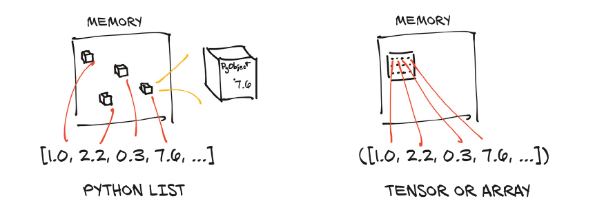
Python’s list stores each list’s member (object) in uncontigious memory block. Then the Python list references these memory address to construct a list. Whereas, a tensor’s values are stored in contiguous memory block and thus faster access and modification. You may notice that this is the same as the true definition of array, as Pytorch Tensor is written on top of C++.

Tensor also requires all the elements to be in the same data types (same with C/C++ arrays). Thus, easy to maintain and manipulate underlying data. For example, 100 32-bit (4 bytes) float elements will consume 800 contiguous bytes, plus some overhead for metadata, on the memory.

II. Tensor creation and its API

Here, we would be introduced with different methods to create a Tensor, as well as some awesomes APIs that Tensor offer to do tensor computations.

1. Constructing a Tensor

We can easily create a Tensor from lists and tuples (must be the same type) by using torch.tensor

a = torch.tensor([1,2,3]) # From Python list
a1 = torch.tensor([[1,2,3],[4,5,6],[7,8,9]]) # Python multidimensional list
a3 = torch.tensor((1,2,3))

print(f"From Python list:\n {a}")
print(f"Python multidimensional list:\n {a1}")
print(f"Python tuple:\n {a3}")

From Python list:
 tensor([1, 2, 3])
Python multidimensional list:
 tensor([[1, 2, 3],
        [4, 5, 6],
        [7, 8, 9]])
Python tuple:
 tensor([1, 2, 3])

We can also create a tensor from numpy.array with torch.from_numpy or torch.tensor.

import numpy as np

a = np.array([1,2,3,4])
a_t_1 = torch.tensor(a)
a_t_2 = torch.from_numpy(a)

print(f"Tensor from torch.tensor:\n {a_t_1}")
print(f"Tensor from torch.from_numpy:\n {a_t_2}")
print(a_t_1 == a_t_2)

Tensor from torch.tensor:
 tensor([1, 2, 3, 4])
Tensor from torch.from_numpy:
 tensor([1, 2, 3, 4])
tensor([True, True, True, True])

We can also use methods from torch to create specials Tensors or from range like Python or even randomly.

# Create Tensors from ones or zeros.
a = torch.ones((2,2)) # (2,2) is the shape of the Tensor. We will discuss this later.
print(f"Tensor with ones:\n {a}")
b = torch.zeros((2,2)) # Similarly, tensor with zeros.
print(f"Tensor with zeros:\n {b}")

Tensor with ones:
 tensor([[1., 1.],
        [1., 1.]])
Tensor with zeros:
 tensor([[0., 0.],
        [0., 0.]])

# We have seen before how to create tensor from list
a = torch.tensor([[1., 2.], [3., 4.]])
print(a)

b = torch.arange(0, 5, 2) # torch.arange() is similar to list's range()
print(b)

tensor([[1., 2.],
        [3., 4.]])
tensor([0, 2, 4])

Pytorch has provided us many useful APIs to easily compute many operations. Most of the operations can be found under the hood of the torch module.

# Calculate the mean
a = torch.arange(0., 6.)
mean = torch.mean(a)
print(f"Mean of {a}: {mean}")

Mean of tensor([0., 1., 2., 3., 4., 5.]): 2.5

# Calculate std
a = torch.arange(0., 6.)
torch.std(a)

tensor(1.8708)

# Transpose a matrix
a = torch.rand((2,3))
print(f"Before:\n {a}")

a_t = torch.transpose(a, 0, 1)
print(f"After transpose:\n {a_t}")

Before:
 tensor([[0.0453, 0.9888, 0.5636],
        [0.0724, 0.8273, 0.8851]])
After transpose:
 tensor([[0.0453, 0.0724],
        [0.9888, 0.8273],
        [0.5636, 0.8851]])

These operations can also be called as a method of the Tensor object.

# Calculate mean using method
a = torch.arange(0., 6.)
a.mean()

tensor(2.5000)

# Calculate std
a = torch.arange(0., 6.)
a.std()

tensor(1.8708)

# Transpose a matrix
a = torch.rand((2,3))
print(f"Before:\n {a}")
a.transpose(0, 1)

Before:
 tensor([[0.7853, 0.4437, 0.4190],
        [0.5611, 0.9481, 0.8179]])

tensor([[0.7853, 0.5611],
        [0.4437, 0.9481],
        [0.4190, 0.8179]])

2. Tensor APIs

The APIs not only offers to create Tensors and compute operations, they also give us information about the Tensor, such as the storage of the Tensor in the memory, the shape of the Tensor, et cetera.

For example, we can get the shape of the Tensor, which is similar to the terminology “dimension”.

# The shape of the tensor
a = torch.rand((2,3))
a

tensor([[0.5457, 0.4495, 0.8650],
        [0.8187, 0.3386, 0.5432]])

a.shape # This returns (2,3)

torch.Size([2, 3])

# View storage offset of Tensor
a = torch.rand((2,3))
a.storage_offset()

In summary, there are many kinds of provided APIs by Pytorch:

Creation ops: Functions for constructing a tensor, such as torch.ones
Indexing, slicing, mutating ops: Funtions to change the shape, stride, or content of the tensor, such as torch.transpose
Math ops: Functions to manipulate the content of tensors through computations
Random Sampling: Functions for generating random values
Serialization: Functions for saving and loading tensors
Parallelism: Functions for controlling the threads of the CPU execution.

These maybe unfamiliar with you, but we promised to be back on these APIs later.

# Create a random tensor
a = torch.rand((3,3)) # Similar to Python random.rand()
print(a)

b = torch.randint(high=5, size=(3,3))
print(b)

tensor([[0.8989, 0.0381, 0.9239],
        [0.8246, 0.9186, 0.8113],
        [0.8812, 0.0537, 0.7803]])
tensor([[3, 3, 1],
        [2, 0, 3],
        [4, 0, 0]])

III. Tensor indexing and slicing

Pytorch’s Tensor indexing and slicing is identical to Numpy Array’s. Therefore, if you are familiar with Numpy’s Array, skip to the next section or you may keep reading if a refresh is needed on this topic.

Just to remind readers, we will take a look at Python list indexing then slicing. Tensor’s approach is similar, but it is far more powerful and efficient.

a = [1,2,3,4]
print(a)
print(f"Item at index 0: {a[0]}") # Item at index 0
print(f"Item slicing from start to index 2 (exclusive): {a[:2]}")
print(f"Item slicing from index 2 to the end): {a[2:]}")

[1, 2, 3, 4]
Item at index 0: 1
Item slicing from start to index 2 (exclusive): [1, 2]
Item slicing from index 2 to the end): [3, 4]

Python indexing pattern is

list[index]

where index can be positive (from 0 to length of the list - 1) or negative (-1 at the last element, -2 at the second last, et cetera).

Whereas, Python slicing pattern can be summarize as:

list[start:end:step]

where

start: the beginning index of the slice (inclusive).
end: the ending index of the slice and EXCLUSIVELY.
step: The step of the slice. Default is 1. If the step is n, the next index to include is i + n.

More examples on negative indexing and slicing:

print(a[-1]) # Last element
print(a[:-1]) # Get the list exclude the last element

4
[1, 2, 3]

We can then apply the same intuition to Pytorch tensor.

a = torch.tensor([1.,2.,3.,4.,5.])
print(a[-1]) # Negative inexing (get the last element)
print(a[0]) # Get the first element
print(a[:3]) # Get a slice from the first element to the third element

tensor(5.)
tensor(1.)
tensor([1., 2., 3.])

Pay attention to the return results of the slices. They are all tensor, include the scalar values such as tensor(5.). Slicing a tensor always return a tensor, although the underhood memory is not change, the return tensor is another view of the origin tensor.

We can easily index a Tensor by using the following snippet:

tensor[dim0-index, dim1-index,..., dimn-index]

where an index can be positive or negative as discussed in Python list indexing topic.

We can also do a multidimensional slice with following pattern:

tensor[dim0-slice, dim1-slice, ..., dimn-slice]

where a dim-i-slice is identical to Python slicing method and we can skip from dim-i-slice to dimn-slice if we decide to get all the elements that contained in the dimensions between i and n.

You may not be familiar with tensor’s dim. If you have a mathematics background, an n-dim tensor would be similar to an n-dim matrix, whereas a computer scientist would tell that it is an N-D array.

For example,

a = torch.rand((2,3,4))
print(f"Origin tensor:\n {a}")
print("Slicing:")
print(a[:,:,:]) # Return the origin tensor

print("Get the first index of dim0, then get from index 1 of dim1, then all of dim2")
print(a[0,1:,:])

Origin tensor:
 tensor([[[0.6342, 0.2091, 0.7519, 0.4431],
         [0.0158, 0.0384, 0.4566, 0.8862],
         [0.7682, 0.8564, 0.7546, 0.8692]],

        [[0.1078, 0.8791, 0.1531, 0.6164],
         [0.9491, 0.3946, 0.9780, 0.4464],
         [0.1266, 0.8538, 0.5849, 0.4837]]])
Slicing:
tensor([[[0.6342, 0.2091, 0.7519, 0.4431],
         [0.0158, 0.0384, 0.4566, 0.8862],
         [0.7682, 0.8564, 0.7546, 0.8692]],

        [[0.1078, 0.8791, 0.1531, 0.6164],
         [0.9491, 0.3946, 0.9780, 0.4464],
         [0.1266, 0.8538, 0.5849, 0.4837]]])
Get the first index of dim0, then get from index 1 of dim1, then all of dim2
tensor([[0.0158, 0.0384, 0.4566, 0.8862],
        [0.7682, 0.8564, 0.7546, 0.8692]])

IV. Tensor element types

As discussed, a tensor only contains elements with the same type, which means, you cannot have a tensor with both float and int as your element types. It is the same as lower programming language’s array but this approach proved to be move optimal than Python’s implementation of list although it is more incovenient for beginners.

Moreover, Pytorch also use a self-implement type formats for numbers, called as dtype. This solve lots of problems raised by standard Python numeric types as below:

Numbers in Python are objects: Although a floating-point number only requires 32-bit on the memory, Python would convert it into an object with reference counting, and so on. This is called boxing and add overheads to the memory. If storing a small amount of number, this is not a problem, but a large amount such as millions would raise an issue.
Lists of Python are created for sequential objects: Lists are not created for mathematics operations. Therefore, there is no method to efficiently add two lists or do a transpose or multiply lists.
Python interpreter is slow compared to an optimized, compiled code. Running a C program takes less less time than a Python program.

As a result, Pytorch introduce dedicated data structure (Tensor), which is a low-level implementations of numerical data structures and relational operations on them, and finally wrap them on a higher-level API. Since they are low level, the elements must be the same type and Pytorch keeps track of them.

1. Specifying different Pytorch’s dtype

a) List of `dtype`

There are many different Pytorch’s dtypes, as listed on the documentation:

32-bit floating point: torch.float32 or torch.float
64-bit floating point: torch.float64 or torch.double
64-bit complex: torch.complex64 or torch.cfloat
128-bit complex: torch.complex128 or torch.cdouble
16-bit floating point: torch.float16 or torch.half
16-bit floating point: torch.bfloat16
8-bit integer (unsigned): torch.uint8
8-bit integer (signed): torch.int8
16-bit integer (signed): torch.int16 or torch.short
32-bit integer (signed): torch.int32 or torch.int
64-bit integer (signed): torch.int64 or torch.long
Boolean: torch.bool

b) Specify `dtype` when create new Tensor

We can specify the dtype of the Tensor while creating the Tensor by giving the value of the dtype to the dtype argument of the constructor.

a = torch.zeros(5, dtype=torch.float32) # Default dtype is torch.float32
a

tensor([0., 0., 0., 0., 0.])

a = torch.zeros(5, dtype=torch.int8) # Specify an torch.int8 tensor
a # Notice the elements are 0 not 0.

tensor([0, 0, 0, 0, 0], dtype=torch.int8)

a = torch.zeros(5, dtype=torch.bool) # Specify a boolean tensor
a # Elements are false

tensor([False, False, False, False, False])

# We will check if the elements have the same dtype
a = torch.zeros(5, dtype=torch.int8)
for i, val in enumerate(a):
  print(f"element {i}: dtype: {val.dtype}")

element 0: dtype: torch.int8
element 1: dtype: torch.int8
element 2: dtype: torch.int8
element 3: dtype: torch.int8
element 4: dtype: torch.int8

2. Choosing the correct dtype

By default, tensor’s element values’ dtype is torch.float32. This normally works well in almost all occasion in deep learning by provide a good precision to the models but also a good speed. You can also increase the precision of the number by setting the dtype to torch.float64 which will also increase the accuracy of the model at the cost of computing time and memory. A lower version of floating-point number, torch.float16 is only available on modern GPU. This dtype will decrease the footprint of the model for a minor decrease on the model’s accuracy.

Moreover, a torch.bool dtype tensor can be use to index a tensor with the same shape by applying the following snippet:

tensor1[bool-tensor]

a = torch.tensor([True, False, True])
b = torch.tensor([2,1,3])
c = b[a] # Returns tensor([2,3])
c

tensor([2, 3])

3. Managing `dtype` attribute

We can use the dtype attribute of the Tensor object to check the what dtype our tensor is.

a = torch.rand(5)
a.dtype # Default dtype is torch.float32

torch.float32

b = torch.randint(high=5, size=(2,2), dtype=torch.int8)
b.dtype

torch.int8

We can also change the Tensor dtype to another by using Tensor.to() method or the built-in methods such as Tensor.double() or Tensor.short()

a = torch.rand(5)
print("Before")
print(a.dtype) # Default dtype is torch.float32
print(a)
new_a = a.to(dtype=torch.int16)
print("After")
print(new_a.dtype)
print(new_a)

Before
torch.float32
tensor([0.5833, 0.5485, 0.4965, 0.5713, 0.5079])
After
torch.int16
tensor([0, 0, 0, 0, 0], dtype=torch.int16)

a = torch.zeros(5)
print("Before")
print(a.dtype) # Default dtype is torch.float32
print(a)
new_a = a.to(dtype=torch.bool)
print("After")
print(new_a.dtype)
print(new_a)

Before
torch.float32
tensor([0., 0., 0., 0., 0.])
After
torch.bool
tensor([False, False, False, False, False])

While doing computations on different dtype tensors, the resulting tensor dtype would be the largest dtype value of the component tensors.

points_64 = torch.rand(5, dtype=torch.double)
points_short = points_64.to(torch.short)
points_64 * points_short # dtype=torch.float64

tensor([0., 0., 0., 0., 0.], dtype=torch.float64)

V. How Tensor work: A view into the memory

1. Storage

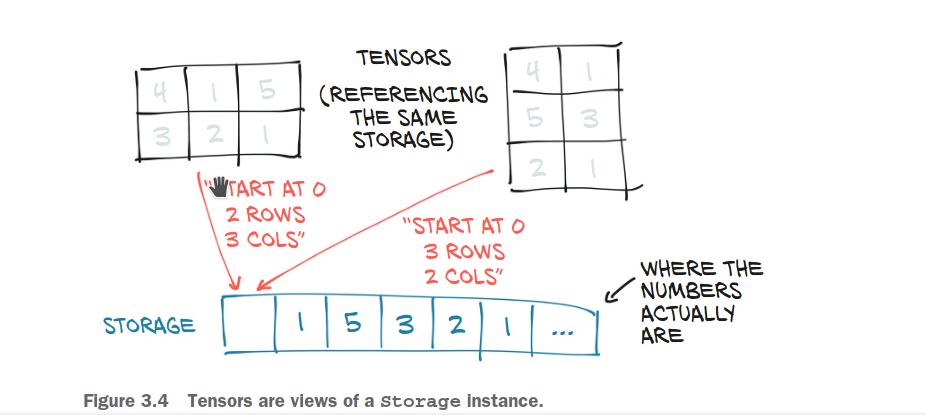
Values in a Tensor are stored in a contiguous chunk in the memory, under the management of an torch.Storage instance. A storage is an one-dimensional array. Thus, the stored values would have the same dtypes.

a = torch.rand(3,3)

a.storage()

4070585370063782
7844629287719727
17825782299041748
15168511867523193
0040580034255981445
6674222946166992
307611882686615
4189969301223755
280387282371521
[torch.storage.TypedStorage(dtype=torch.float32, device=cpu) of size 9]

Although the Tensor has the shape of (3,3), but the underlying Storage would be an one dimensional array of size 9.

Storage

Moreover, multiple Tensor can index one instance of torch.Storage. For example,

a = torch.tensor([[1,2,3],[4,5,6]])
a

tensor([[1, 2, 3],
        [4, 5, 6]])

b = a.transpose(1,0)
b

tensor([[1, 4],
        [2, 5],
        [3, 6]])

We created a new Tensor a, and its transpose b.

a.storage()

 1
 2
 3
 4
 5
 6
[torch.storage.TypedStorage(dtype=torch.int64, device=cpu) of size 6]

b.storage()

 1
 2
 3
 4
 5
 6
[torch.storage.TypedStorage(dtype=torch.int64, device=cpu) of size 6]

We can see that the values and their orders in the Storage objects are the same. And sinve we mentioned that, “Tensor indexes Storage”, we actually mean it. Storage objects can be indexed in the way similar to list:

a.storage()[0]

But note that Storage cannot be sliced through:

a.storage()[:3]

---------------------------------------------------------------------------

RuntimeError                              Traceback (most recent call last)

<ipython-input-38-e634286c0d18> in <module>
----> 1 a.storage()[:3]


/usr/local/lib/python3.8/dist-packages/torch/storage.py in __getitem__(self, idx)
    524         # so it was disabled
    525         if isinstance(idx, slice):
--> 526             raise RuntimeError('slices are only supported in UntypedStorage.__getitem__')
    527         elif not isinstance(idx, int):
    528             raise RuntimeError(f"can't index a {type(self)} with {type(idx)}")


RuntimeError: slices are only supported in UntypedStorage.__getitem__

At this point, many readers may ask, “What if we modify a value of torch.Storage instance? This is a good question. We can modify the value of a Storage instance. Since Storage stores the values of the Tensors, changing the values of the Storage also change the corresponding values of the Tensors.

# Recall a matrix
a

tensor([[1, 2, 3],
        [4, 5, 6]])

# Changing number 2 to 10
a.storage()[1] = 10

tensor([[ 1, 10,  3],
        [ 4,  5,  6]])

The value 2 of Tensor a changed to 10! More interestingly, another Tensor has its value changed! You guessed it right! Tensor b’s 2 also changed to 10 as they share the underlying Storage.

tensor([[ 1,  4],
        [10,  5],
        [ 3,  6]])

There are many operations that modify the values of the underhood Storage, and they are called in-place operations.

2. Tensor metadata: Size, strides, and offset.

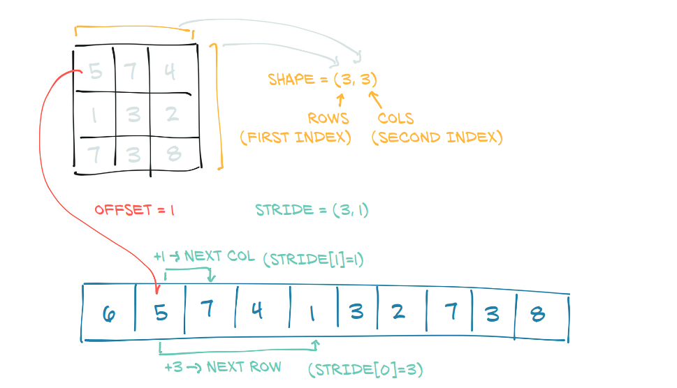
The size of a Tensor, is a tuple represents the number of elements in the corresponding dimension. For instance, a size (3,2) represents a Tensor that would have 3 elements at dimension 0, 2 elements in dimension 1.

The storage offset represents the index of an element in the Storage object, which is the first element in the corresponding Tensor.

The stride is a tuple, which values represent the number of elements should be skipped to get the next elements in the Tensor per dimension.

Size, offset, stride

tensor([[ 1, 10,  3],
        [ 4,  5,  6]])

a.storage()

 1
 10
 3
 4
 5
 6
[torch.storage.TypedStorage(dtype=torch.int64, device=cpu) of size 6]

The size of a shows that the Tensor has 2 rows and 3 columns.

a.size()

torch.Size([2, 3])

Since the first element of a is 1, which is also the first element of the Storage, the return value is indeed 0.

a.storage_offset()

Let’s look closer at the stride of a. The return value is (3,1). Which means the number of elements to skip the get the next value at dimension 0 is 3, while dimension 1 is 1.

For easier interpretation, let’s call dimension 0 a row, and dimension 1 a column. Then, everything is clearer now, to get the element at the next column, we must skip to the next element in the Storage (for example, the next column’s value of 1 is 10, which is also the next value in the Storage), and since a row contains 3 values, the value in the next row is obtained by skipping the next 3 elements in the Storage.

a.stride()

(3, 1)

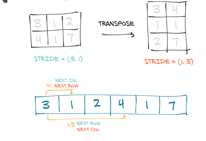
Therefore, changing the offset and the stride changes a Tensor completely, while different Tensors can be built on top of a Storage based on different values of offsets and strides.

a.stride()

(3, 1)

b.stride()

(1, 3)

For example, changing 2 values in the stride gives a transposed Tensor.

Transpose a Tensor

VI. CPU and GPU

One can change a Tensor from CPU to GPU using:

a.cuda()

tensor([[ 1, 10,  3],
        [ 4,  5,  6]], device='cuda:0')

a.to(device="cuda")

tensor([[ 1, 10,  3],
        [ 4,  5,  6]], device='cuda:0')

Or from GPU to CPU:

a.cpu()

tensor([[ 1, 10,  3],
        [ 4,  5,  6]])

a.to(device="cpu")

tensor([[ 1, 10,  3],
        [ 4,  5,  6]])